Wednesday, December 29, 2010

Catchup Post: Graphics

ShaderToy
Another set of interesting links:

Friday, December 24, 2010

Humble Bundle #2 - Great indy games - name your price!

Osmos - Humble Bundle 2
The independent games humble bundle offer is back again, better than before. It is a pay-what-you-want offer for 5 indy games, all of which have support for Windows, Mac OSX and Linux. If you pay above the average, you get the previous humble-bundle pack of 6 games as well! A very good deal for whatever you want to pay! (Makes an excellent Christmas present!) Anyone studying games design or games programming should get these games to learn from them - what works, what doesn't? Braid is a fabulous example of teaching the player the game without needing to give them a tutorial, and many of these games are great examples of the scope you should aim for if you are making your own game.

The games included are:
  • Braid - a side scrolling puzzle/adventure through time. Nicely designed gameplay.
  • Cortex Command - side scroller, not very impressive.
  • Machinarium - a point and click adventure game, nice graphics, pretty decent.
  • Osmos - an ambient physics-based "eating" game (you absorb smaller entities). Good gameplay and a great "programmer-game" (nice graphics). My pick of the lot. (only $10 separately)
  • Revenge of the Titans - a tower-defense (build towers that destroy enemies) game. Nothing special.
The other games are:
  • World of Goo - a construction puzzle game. Lots of fun.
  • Aquaria - an underwater fantasy game.
  • Gish - a platform game.
  • Lugaru - 3D action adventure game.
  • Penumbrac - a FPS/adventure game.
  • Samorost 2 - a flash-based puzzle game.
If you pay 10 USD to get them all, that works out to less than a dollar a game, and I guarantee you will find at least one game you think is worth $10 in the humble (cross-platform games) bundle.

Thursday, December 23, 2010

Underground

Few updates this month because I've been underground. And I don't mean I've joined some kind of strange sub-culture or gone in hiding, I mean literally 1.5km vertically underground to commission a Transmin automated Rockbreaker (there's not much internet down there!). A few things I learnt / experienced about hard-rock underground mines (most of which are very obvious):
  • Block caving is insane. The idea is to create an extraction level under the ore body, then continuously blast the ore into smaller rocks that can be processed, leaving a massive growing "sink" hole on the surface. You also need a very very very long conveyor belt.
  • The tunnels are quite large, as some very large vehicles need to drive through the mine.
  • All the tunnels have a 'clean' look to them, largely thanks to the use of shotcrete (i.e. concrete reinforcement around the tunnel rock).
  • It takes 45 minutes to drive down to a depth of 1.5km
  • When driving, give way to larger vehicles, or vehicles with explosives.
  • Its difficult to move around quickly, you will easily break a sweat in no time.
  • Batteries weigh a lot when you need to carry them around on a belt all day
  • You use a lot more oxygen if you panic, or move around a lot
  • There is a complex system of ventilation channels with really really big fans providing all the air
  • It is really easy to get lost in a large underground mine
  • There is an underground dining area. It is called the 'crib'. I don't know why.
  • If anything bad happens, you don't have much of a chance, especially if you are not aware of all the intimate details of how the mine operates. (ie: haven't been there for more than a year)
  • Explosions are loud
  • Ground movement is bad and very very loud
  • There is an awful lot of dust
All in all an interesting experience, but all the dust certainly didn't do any good for my eyes or my lungs. I've been coughing a lot even after being out of the mine for a week as the very fine dust just gets everywhere.

Friday, November 26, 2010

XV-11 LIDAR Hacked!

Congratulations to the team at Random Workshop blog, Hash Salehi modified some code from Nicolas Saugnier to parse the LIDAR data in realtime!

Movie follows:


That didn't take long!

Thursday, November 25, 2010

GPGPU catchup

Another month, another catchup post on the world of GPU's. A few interesting things have happened:

Wednesday, November 24, 2010

Microsoft Kinect and other devices

The Microsoft Kinect is a very cheap 3d vision system that provides performance somewhere between stereo cameras and more expensive time-of-flight (eg:PMD) cameras. It was actually something I was hoping would come out before the end of the MAGIC 2010 competition, but unfortunately the release date was scheduled for after the end of the competition.

The device was "hacked" almost immediately after its release and it has already been widely adopted, I think this will do wonders for the robotics/computer vision/stereo-vision community. So far all we have seen are relatively simple applications, but I'm sure people will start pushing the interpretation of the data to its limits soon, especially given that game-developers are now going to be playing with this kind of data. The Wii has already done fantastic things to push the knowledge of filtering and dealing with noisy sensor data to a wider audience, and I expect the Kinect will have a similar effect.

It all started with Adafruit offering $2000 bounty for the Kinect hack, which was promptly won by Hector Martin on the 10th of November.
One of the first videos (now viral!) to do the rounds was from Oliver Kreylos showing the 3d data fused with image data and rendered in OpenGL.


Of course, it didn't stop there, other people are trying to hack the rest of the USB Kinect protocol for the inclinometer and motor controls, and trying to figure out how the Kinect IR works.

Willow Garage has already begun work on integrating the Kinect to ROS including calibration functions, and Philip Robbel managed to integrate the Kinect with a Hokuyo to do visual SLAM (using MRPT) only 7 days after the hack was released.


Hopefully we will see more practical uses for the Kinect soon! Wired published a nice story on the development path at Microsoft of the Kinect.

The best thing about this "hack" is that it has inspired others to do the same, most notably the $800 reward for hacking the Neato Robotics XV-11 vacuum cleaner LIDAR. (Whitepaper here!). At only $300 (or even $30!) for a 360 degree, 6m range, 10Hz scanning LIDAR this would do great things for the robotics community as well. Sparkfun have already made some interesting progress with their LIDAR tear-down.

Exciting times!

Monday, November 22, 2010

Batch import OBJ with Blender

The OBJ importer in blender actually supports batch-import, to enable this you need to hold SHIFT when you select the importer from the File->Import->Wavefront (obj) menu. You will then be prompted to select a directory. Unfortunately, the importer will import each OBJ file into a separate (and incorrectly constructed) scene. To alter this you will need to edit the "import_obj.py" script and comment lines 1164 and 1165:
for f in files:
   #scn= bpy.data.scenes.new( stripExt(f) )
   #scn.makeCurrent()
Saves you from having to write a batch import script yourself! A great utility to convert to OBJ files from various formats (with a batch-convert mode!) is polytrans.

Thursday, November 18, 2010

Team MAGICian/WAMbot takes 4th place!

All of our teams hard work has paid off as we claimed 4th place in the MAGIC 2010 competition! Our system was actually very close to what the top two teams had implemented, and with a bit of luck we might have been able to snatch a prize. Maybe next time!


Above is a photo composition by Rob Reid of all the robots at the challenge stand, ordered from 1st to last (Left to Right). Team Michigan came in 1st, followed by University of Pennsylvania, and RASR took 3rd place. It's been a great opportunity to talk to all the other teams and see how they solved their problems and to see how many of the same headaches we all had. The LWC was a great place to meet and greet a number of industry people and also a nice crowd from DSTO who showed a lot of interest in what we have done. It was great to get so much positive feedback from everyone on our system.

Friday, November 12, 2010

Ram Shed Challenge

The Ram Shed challenge was a media-event for the MAGIC 2010 competition. It was our first chance to see all the other teams robots and a chance to see them all at work. Our robots performed very well one the day and navigated the maze better than any other team, the entire open section of the maze was explored fully autonomously requiring no human interaction at any point. All of this despite the fact our wifi gear was mounted outside and failed during the rain, after a few minutes we were able to replace it and continue our mapping operations!
The photos show our robots at the starting line, followed by them moving off in the starting arena, then navigating the maze, and finally the prize.
A fabulous effort by our team, and I'm extremely proud of our achievements on this day!

Sunday, November 07, 2010

Team MAGICian

Our MAGIC 2010 test day is over, so it's time to catch up on some sleep!
Looking forward to seeing how the other teams will perform.

Sunday, October 31, 2010

MAGIC 2010 - Adelaide

We are off to Adelaide for the MAGIC 2010 finals.
Looking forward to meeting the other teams, and hope it doesn't rain!

Wednesday, October 27, 2010

Convex Hull Generation in Blender

Convex hulls are very useful for a number of optimized calculations such as fast intersection tests, fast spatial subdivision, and other early-out's used in computer graphics, computational physics and robotics.

When I implemented convex hull generation and convex decomposition in PAL I first used qhull and leveraged code from tokamak physics, but then used code by Stan Melax and John Ratcliff for PAL. Recently my work at Transmin has required generation of a number of Convex hulls, and so I combined these snippets of old code to create a plug-in for Blender.

The Blender plugin creates a bounding convex hull of the selected object.
It calls an external executable 'convex' which creates a convex hull based on an intermediate OBJ file.

Installing the plugin requires you to compile the code to generate the 'convex' executable, and copying the python code into Blender's scripts directory.

To compile the C code on linux/osx:
g++ createhull.cpp hull.cpp -o convex

Place the object_boundinghull.py script in your ".blender/scripts" directory.

On OSX Blender default installs to:
/Applications/blender-2.49b-OSX-10.5-py2.5-intel/blender.app/Contents/MacOS

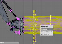
Once the plugin is installed you can start creating convex hulls. You can select an object in blender and cut it into smaller objects to manually decompose the hulls. To do this, you can use the Knife tool (K) or split objects in edit-mode with 'P'. (Selection tools like 'B' and manual alignment of cameras ('N', Numpad 5) will help a lot).

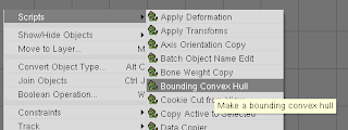
Once you have the objects you would like to generate hulls for select one, and run the "Bounding Convex Hull" script. It will ask you to confirm the creation of the hull. The new hull will have the same name as the original object and have ".hull" appended to its name.

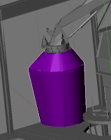
The plugin will generate a new object that represents the convex hull of the selected object, with the same transforms as the original object. (Ctrl-A to apply all down to the mesh, note: Blender 2.49 does not let you apply translation transforms, but Blender 2.5+ does). You can then decimate the hull to reduced the number of tri's used to represent your object. (Editing F9, under modifiers, select 'Add Modifier', decimate, and reduce the ratio).


Now your ready to export your scene for all your raytracing and collision detection needs!

Thanks to Transmin Pty Ltd for allowing me to release this plugin back to the Blender community under the GPL.

Follow the link to download the Blender Bounding Convex Hull plugin to generate editable bounding volumes directly in Blender.

Sunday, October 10, 2010

Using BZR

BZR supports a number of different workflows. The most common one is "Centralized", which allows you to use BZR just like CVS or SVN. You just type "bzr commit" (save changes) and "bzr update" (get changes).

However, BZR has the advantage of being a distributed system and thus gives you the option of branching, working remotely (and still having version control), and then merging your changes back to the main trunk.

You can do this in a few easy steps:
  1. Make a copy of your code, by making a new "branch" of the code. Example:
    (On LOCAL)
    bzr branch WAMbot WAMbotAdriansBranch
    
    In future, you can keep this branch up to date by using "bzr pull" from the branch.
  2. Copy the branch to your target (eg: a robot / embedded PC or usb-stick). If you copy from the USB stick to the target you will need an extra step to go back.
  3. Work with the source code on the target. After you have made changes just type "bzr commit" (on the target). This will commit to your local branch.

    Now you have the advantage of being able to revert any changes that you make while working away, without needing a connection to the main server.
  4. If you copied from the USB stick, and you want to save the changes back to it, type (at the target): "bzr push LOCATION" (Where LOCATION is the USB disk drive). Example:
    (On TARGET)
    bzr push "e:/WAMbotAdriansBranch"
    
    from the bzr directory on the robot.
  5. Now merge with your local repository, from your own bzr directory type:
    bzr merge LOCATION (Where LOCATION is the USB disk drive, or shared folder) Example:
    (On LOCAL)
    bzr merge X:\WAMbotBranch
    
  6. Now you can commit them to the central server! (Just use bzr commit like always)
This saves you from having to keep track of your source code and merge things manually. Some more helpful BZR tips:
  • bzr update (get the latest code from the server)
  • bzr commit (save your code to the server)
  • bzr add (add some files to repo)
  • bzr whoami (get/set who you are)
  • bzr revno (get current revision number)
  • bzr diff -r REVISION (eg: 1000) filename (tells you the differences in a file since a specified revision)

    There are a number of revision flags:
    • bzr diff -r last:5 (compare with 5 revision ago)
    • bzr diff -r date:yesterday (compare with yesterdays revision)
    • bzr diff -r date:YYYY-MM-DD (compare with a dated revision)
  • bzr commit --local (commit to your own local repository, so you can easily undo changes. Note: you may need to bind/unbind, so branching as described above is probably better)
  • bzr revert (undo your changes)
  • bzr log (show commit comments)
  • bzr log -r REVISION.. (show all comments since given revision. Example: "bzr log -r1000..")
BZR also has a number of plugins, including one to run a command before a commit.

Friday, September 24, 2010

Circular Motion in 2D for graphics and robotics

For a number of applications circular motion in 2D is useful, in particular simplified kinematic representations for mobile robot simulation and control. There are a number of different ways of representing this motion.

First it is helpful to remember a position on a circle can be described parametrically by:
[x,y] = [r*cos(theta), r*sin(theta)]
or alternatively, r =sqrt( x^2 + y^2).

  1. As a circular variation of the standard 2D particle, we just add an angular velocity (omega) and angular orientation (theta). For a standard 2D particle we can describe its velocity (v) in terms of acceleration (a) and a delta in time (dt) (v += a*dt; x+= v*dt). We can modify this to include the parametric circle representation:

    theta += omega * dt;
    x+=v*dt*cos(theta);
    y+=v*dt*sin(theta);
    
  2. The problem with the above method is that it is in-exact and relies on an integrator. The 2D velocity/angular velocity representation can easily be fully solved analytically. The radius of a circle produced by a given velocity (v) and angular velocity (omega, or w) is:
    r = | v / w |
    We can modify the parametric representation to include an offset for the centre of motion:
    [x,y] = [r*cos(theta) + xc, r*sin(theta) + yc]
    Thus, given an initial x,y,theta we can find the centre of the circle of motion as:

    xc = x - (v/w)*sin(theta)
    yc = y + (v/w)*cos(theta)
    
    Now we can update the position of the robot:

    theta += w * dt;
    x = xc + (v/w) sin(theta)
    y = yc - (v/w) cos(theta)
    
    We can expand this into a single line as:

    x+= -(v/w)*sin(theta) + (v/w)*sin(theta+w*dt)
    y+= -(v/w)*cos(theta) - (v/w)*cos(theta+w*dt)
    theta += omega * dt;
    
    Which is the form many robotics papers use.
  3. Finally, we may wish to represent the motion in terms of two given x,y coordinates and solve for the translation and rotation required to reach them (as is the case for odometry calculations). In this case, we can represent any movement from an original set of coordinates [x,y,theta] to a new set [x',y',theta'] as first a rotation and translation to bring you to any new x' and y', followed by another rotation to bring you to the final theta'. Using triangle trigonometry this is:

    deltaRot1 = atan2(y'-y,x'-x) - theta
    deltaTrans = sqrt( (x-x')^2 + (y-y')^2 )
    deltaRot2 = theta' - theta - deltaRot1 
    
There are of course many more ways of representing circular motion, but the above are the most common in computer graphics and robotics.

Tuesday, September 14, 2010

Intel Compiler on Linux

  • Make sure you have access to root. (eg: sudo su root, passwd)
  • Make sure you have your build environment set up. eg:

    sudo apt-get install gcc
    sudo apt-get install build-essential
    sudo apt-get install g++
    sudo apt-get install rpm
    
  • ICC requires older standard C libraries, libstdc++5, so you can get them for Ubuntu from:
    Package: libstdc++5. You just need to download the i386 package. (eg from the Australian mirror, by using wget [url]), and then install it, eg: "sudo dpkg -i libstdc++5_3.3.6-18_i386.deb".
    If you don't do this you may get the following error messages:

    Missing critical pre-requisite
    -- missing system commands
    
    The following required for installation commands are missing:
    libstdc++.so.5 ( library)
    
  • Download ICC
  • Unzip (tar -xvf filename)
  • ./install.sh
  • Choose to install for all (1)
  • Read "welcome" message follow instructions for licence, etc.
  • Activate your software (1) and provide the serial number that came in your email. You should see "Activation Completed Successfully"
  • Install the software (requires 3.35 gigs). You should see a message "Checking the prerequisites. It can take several minutes. Please wait…".
  • You might see:

    Missing optional pre-requisite
    -- No compatible Java* Runtime Environment (JRE) found
    -- operating system type is not supported.
    -- system glibc or kernel version not supported or not detectable
    -- binutils version not supported or not detectable
    
    The JRE you need for the visual debugger, otherwise you can safely continue.
  • The installer then asks which components to install, eg "Intel(R) C++ Compiler Professional Edition for Linux*", just press "1. Install" to continue. It should state "component installed successfully."
  • Setup the paths, you can use the iccvars.sh in /opt/intel/Compiler/11.1/073/bin to setup everything for you. (eg: source /opt/intel/Compiler/11.1/073/bin/iccvars.sh ia32). You may wish to put it into your .bashrc file.
  • That's it! Type "icc" to invoke for C files or "icpc" for C++ files. For standard makefiles use "make CXX=icpc"
On a 1GHz VIA Esther processor, GCC 4.4.1, with -O2 -march=c3-2:
real 0m16.855s
user 0m16.849s
sys 0m0.004s
And, with ICC 11.1, with -O2:
real 0m11.369s
user 0m11.361s
sys 0m0.008s

An instant 45% speedup! Unfortunately not all code makes such a big change, some other compute-intensive code I tested only got a 4% speedup. In any case I'd say its worth it!

Sunday, September 12, 2010

SIGGRAPH 2010 Course Papers Overview

I've managed to work through the SIGGRAPH 2010 course content that relates to realtime rendering. I quite liked the Toy Story 3 rendering techniques and realtime rendering survey by nVidia- just because they give a nice overview. As always, there are a number of great presentations, and I've listed the ones that I found interesting below.
  • Toy Story 3 : The Video Game Rendering Techniques from Avalanche Software gives a great (211 page!) overview of a number of lighting issues for the game including SSAO (various optimizations/approximations for how/where to sample, faking more samples and dealing with large differences in depth), ambient lighting (without needing to bake it or do GI) and various aspects on shadows. A great read!
  • Surveying Real-Time Rendering Algorithms by David Luebke from nVidia gives an excellent short overview of a number of recent developments in realtime rendering algorithms including stochastic transparency (ie : transparency via random sampling), sample distribution for shadow maps (partitioning the scene in light-space), alias-free shadow maps, append-consume order-independent-transparency (sorting per-pixel & linked-lists), progressive photon mapping, image-space photon mapping, ambient occlusion volumes (how to speed it up with bitwise occlusion mask for each triangle - one per edge, and one for the triangle plane), stochastic rasterization (of 4d triangles)
  • Keeping Many Cores Busy: Scheduling the Graphics Pipeline by Jonathan Ragan-Kelly from MIT gives a great overview of the graphics pipeline stages (from Input Assembler, Vertex Shader, Primitive Assembler, Tesselation, Geometry Shader, Rasterizer, Pixel Shader, and finally Output Blending) and load balancing.
  • Uncharted 2 - Character Lighting and Shading by John Hable from Naughty Dog gives a fabulous overview of rendering issues with skin (in a lot of detail!), hair and clothes.
  • Bending the Graphics Pipeline by Johan Andersson from DICE describes tile-based deferred shading (for GPU and SPU), morphological antialiasing and analytical ambient occlusion.
  • A real-time Radiosity Architecture for Video Games by Sam Martin and Per Einarsson from DICE/Geomerics introduce the 'Enlighten' system for realtime GI - it gives a nice overview.
  • Evolving the Direct3D Pipeline for Real-­time Micropolygon Rendering by Kayvon Fatahalian from Stanford University gives an interesting insight on Micropolygon rendering on current GPU pipelines.
  • Water Flow in Portal 2 by Alex Vlachos - I've already written about this previously, just another realtime technique for faking the simulation and rendering of water flow.
  • Making Concept Real For Borderlands by Gearbox Software contains some nice examples of their concept art, the development change from photorealistic to stylistic rendering and art (and the code/artist balance), and the sobel edge filter they used.
  • The notes from the volumetric course was broken into parts:

    1. "Resolution Independent Volumes" - which describes the "Field Expression Language Toolkit", cloud modelling (via density displacement), morphing objects (by using the Nacelle Algorithm to generate warp fields), cutting models, fluid dynamics, gridless advection, and semi-lagrangian mapping (balancing between grids and non-grids).
    2. "Mantra Volume Rendering" - this describes the volume rendering engine for Houdini.
    3. "Volumetric Modeling and Rendering" describes the volumetrics library/API developed at Dreamworks.
    4. "Double Negative Renderer B" (used in Batman Begins, Harry Potter, etc.) describes the workflow and various shaders (Fluid, Particle, Voxel, Fire, Smoke) in DNB
    5. "Volume Rendering at Sony Pictures Imageworks". The section from Sony Imageworks included an overview of their pipeline and content on their open source field/fluid tools.

Wednesday, September 08, 2010

Catchup Post: Graphics & GPU's & Physics

A long overdue catchup post for various interesting things I've spotted over the last two or three months. SIGGRAPH recently finished, so it really deserves a round-up, although I haven't had time to review all the interesting things.
The annual tutorial on
realtime collision had some interesting presentations, I quite liked the one from Erwin Coumans (Bullet) this year - it gives a good overview of the recent advances in the Bullet engine including the GPU optimizations. Simon Green also has a presentation on CUDA SPH rendering (also see Jihun Yu's particle fluid surface reconstruction) and another open source GPU SPH simulation from HPC lab.
The realtime graphics tutorial, stylized rendering, volumetrics, and programmable shaders has some great stuff that I'll look into in more detail in a future post. Ofcourse there is also always the SIGGRAPH 2010 papers list, and SIGGRAPH asia papers (again more on this later..).

Some GPGPU software/links:
and MPTL is a parallel version of the STL algorithms.


Some physics links:
Some graphics links:
And finally a documentary on the history of the Future Crew demo group and Second Reality. Brings back the memories.

Wednesday, August 25, 2010

Kalman filters - Part 2

In a previous post I described kalman filters and gave a very simple example of a 1D filter implemented in C. In the real world, having a filter with three or more inputs is common. A standard 3rd order example would be a filter that considers the position, velocity and acceleration of a system.

In this case you would have a 3x3 measurement matrix (H) (with the diagonal set to what you can measure), a 3x3 process noise matrix (Q), a 3x3 measurement noise matrix (R), and a 3x3 state transition matrix. The standard transition matrix would simply contain v+=a*dt, x+=v*dt, but we can use a 2nd order leapfrog integrator to get better accuracy of our position from our acceleration data. So in total we have:


You can either solve this using the standard kalman matrix maths, but you will find that an SVD approach will give you more stable solutions. OpenCV is one library that already has the kalman matrix maths built in. To set up a kalman filter with OpenCV we just need to setup the matrices we need and call the appropriate cvKalman functions.

(ugly) Code snippet follows:
#ifndef KALMAN_H
#define KALMAN_H

/** OpenCV Kalman filter for 1st, 2nd and 3rd order position, velocity and acceleration data.
    (c) Adrian Boeing
    www.adrianboeing.com
 */
#include <cv.h>

typedef enum {
    K_P = 1, //position only
    K_V = 2, //velocity only
    K_A = 4, //acceleration only
    K_PV = 3, //position & velocity
    K_PA = 5, //position & acceleration
    K_VA = 6, //velocity & acceleration
    K_PVA = 7 //position, velocity and acceleration
} Kalman_e;

class KalmanPVA {
public:
    KalmanPVA(int order, Kalman_e type, float initial_pos, float initial_vel, float initial_accel, float dt, float process_noise[3], float measurement_noise[3]) {
        m_order = order;
        //create the OpenCV kalman structures
        kalman = cvCreateKalman(order, 3, 0 );
        z = cvCreateMat(3,1,CV_32FC1);
        
        //construct the transition matrix
        SetDT(dt);
        
        //enable only the measurements we have!
        for (int i=0;i<m_order;i++) {
            cvmSet(kalman->measurement_matrix,i,i,((type&7)>>i)&1);
        }
        //configure the process noise matrix
        cvSetIdentity( kalman->process_noise_cov,    cvRealScalar(1) ); //zero the matrix 
        for (int i=0;i<m_order;i++) {
            cvmSet( kalman->process_noise_cov,i,i, process_noise[i] ); 
        }
        //configure the measurment noise matrix
        cvSetIdentity( kalman->measurement_noise_cov, cvRealScalar(1) ); //zero the matrix
        for (int i=0;i<3;i++) {
            cvmSet(kalman->measurement_noise_cov,i,i,measurement_noise[i]);
        }
        cvSetIdentity( kalman->error_cov_post,cvRealScalar(10) ); //large initial unknown
        
        //setup the initial state
        cvmSet(kalman->state_post,0,0,initial_pos );
        if (m_order>1)
            cvmSet(kalman->state_post,1,0,initial_vel);
        if (m_order>2)
            cvmSet(kalman->state_post,2,0,initial_accel);
        
        
    };
    void SetDT(float dt) {
        //3rd, 2nd, and 1st order transition matrix models
        
        //3rd order uses 2nd order leapfrog integration
        float F3[] = {   1, dt, 0.5*dt*dt,
            0,  1, dt,
            0,  0,  1};
        
        float F2[] = {   1, dt, 
            0,  1};
        
        float F1[] = {1};
        
        switch (m_order) {
            case 3:
                memcpy( kalman->transition_matrix->data.fl, F3, sizeof(F3));
                break;
            case 2:
                memcpy( kalman->transition_matrix->data.fl, F2, sizeof(F2));
                break;
            case 1:
                memcpy( kalman->transition_matrix->data.fl, F1, sizeof(F1));
                break;
        }
    }
    void SetMeasurements(float pos, float vel, float accel) {
        cvmSet(z,0,0,pos);
        //if (z->rows>1)
            cvmSet(z,1,0,vel);
        //if (z->rows>2)
            cvmSet(z,2,0,accel);
    }
    
    void Update(){
        const CvMat* y = cvKalmanPredict( kalman, 0 );
        cvKalmanCorrect( kalman, z );
    }
    float GetPositionEstimate() {
        float v = cvmGet(kalman->state_post,0,0);
        return v;
    }
    float GetVelocityEstimate() {
        if (kalman->state_post->rows>1)
            return cvmGet(kalman->state_post,1,0);
        return 0;
    }
    float GetAccelerationEstimate() {
        if (kalman->state_post->rows>2)
            return cvmGet(kalman->state_post,2,0);
        return 0;
    }
    float GetPositionError() {
        return cvmGet(kalman->error_cov_post,0,0);
    }
    CvKalman* kalman; //openCV Kalman filter
    CvMat* z; //measurement matrix
private:

    void cvKalmanNoObservation() { 
        cvCopy(kalman->error_cov_pre, kalman->error_cov_post); 
        cvCopy(kalman->state_pre, kalman->state_post); 
    } 
    int m_order;
    
};

#endif

Tuesday, August 17, 2010

CAD packages

Some basic knowledge of CAD packages never hurt anyone. Two of the most common ones used in industry are AutoCAD and SolidEdge. Most of the time you will just need to take measurements from some diagrams rather than build a complete model.

AutoCAD has a command line interface (from way back in the DOS days). Two useful commands for measurement are:
  • di - Measure a distance between two points
  • id - Print the coordinates of a point of interest

Other things you might find yourself doing include drawing lines and circles, which are all relatively self-explanatory. Occasionally you need to measure something relative to a reference line or base line that you want to project through the whole drawing. You can do this by using the 'extend' option to lengthen the line. Simply choose the 'Extend' option from the modify menu and draw a line to represent the boundary of the lines extension, right click, and select the line you wish to lengthen. AutoCAD will lengthen the selected line up to the boundary you specified.

Like Photoshop AutoCAD also has layers which you can work with. You can turn layers on/off by clicking on the lightbulb function.


With SolidEdge you can use the dimension menu to make measurements (Make sure you are working on the correct sheet!). These can be either horizontal/vertical, by two points, or you can select an element in the drawing to use as the axis (easier than in Autocad!).

Friday, August 06, 2010

Computing events in Perth

GameJam is on again in Perth - I didn't see much about it this time, but it is in Joondalup again. Also, there is a GPU computing workshop on the 19th of August in the ARRC auditorium. More information on the workshop is available here.

Thursday, August 05, 2010

A star (A*) pathplanning

Previously I wrote about Dijkstra, this time I'm going to look at heuristic or "AI" style approach the A* algorithm. This is a single-source single-goal pathfinding algorithm. In essence this algorithm "guesses" or estimates the distance that remain to get from a node to the destination node. These estimates guide the direction of the path (i.e. search), with each node that is visited updating the true cost of the path, until a solution is found.

A* considers what to do at each node depending on an overall heuristic score. The total score is a function of the cost of the path that has already been traversed (the "g" cost) and the estimated cost of traveling from the node to the destination (the "h" cost). There are many ways to estimate the "h" cost, typically for pathfinding problems the euclidian distance is used, however it is always better to over-estimate the remaining cost (so you will explore more feasible solutions), and so a common measure used is the manhattan distance.

The A* algorithm works on two lists, a "Closed" list of already explored nodes, and an "Open" list of nodes yet-to-be-explored.

In essence the algorithm is:
  • Select a source node to operate with (eg: the start node, or the node with the lowest overall cost)
  • For each node connected to the source node:
    • Calculate the already-traveresed cost
    • If the node is on the closed list, and the newly calculated traversed cost exceeds the existing traversed cost for the node, skip the node, otherwise remove it from closed.
    • Calculate the estimate cost to find the total cost, and store all these costs with the node.
    • Add the node to the Open list
  • Add the source node to the Closed list
In Pseudo-Code (from Bryan Stout):
priorityqueue Open
 list Closed 
s.g = 0 // s is the start node 
s.h = GoalDistEstimate( s ) 
s.f = s.g + s.h 
s.parent = null 
push s on Open 
while Open is not empty 
  pop node n from Open // n has the lowest f 
  if n is a goal node 
    construct path 
    return success 
  for each successor n' of n 
    newg = n.g + cost(n,n') 
    if n' is in Open or Closed, and n'.g < = newg 
      skip 
    n'.parent = n 
    n'.g = newg 
    n'.h = GoalDistEstimate( n' ) 
    n'.f = n'.g + n'.h 
    if n' is in Closed 
      remove it from Closed 
    if n' is not yet in Open 
      push n' on Open 
  push n onto Closed 
return failure // if no path found 
A great interactive demonstration program can be found here: http://www.policyalmanac.org/games/aStarTutorial.htm And some source code for A* is available from the GrinningLizard website (The same author as the fantastic tinyXML library!) Keep in mind that waypoint-based AI navigation for games is a very mid-nineties approach, nav-mesh's are certainly the way to go! For an example of issues with waypoint approaches take a look at this video: Your best bet for navmesh research is Mikko Mononen's blog.

Wednesday, August 04, 2010

Using Parallel Reduction to Optimize Dijkstra

In a previous blog post I wrote about Dijkstra's algorithm. One optimisation to the naive implementation is to calculate the minimum cost node in parallel - since this can often be the most time consuming operation for large graphs. This is a perfect candidate for a parallel reduction operation.

In serial, if we wished to sum up an array (x) of numbers, the code would be:
int sum = 0;
for(int i=0; i < N; ++i) 
 sum += x[i];

However, in parallel we could speed this up by summing parts of the array and then adding those parts together. For example, to add four numbers a,b,c,d we could first add a+b and c+d in parallel, then sum ab+cd. This is called a 'reduction' operation, and it allows us to complete an otherwise O(N) operation in O(log(N)) steps.

One particularly nifty pattern is the "Butterfly" pattern of adding elements. Best described with an animation:


In code this can be done as:
for (b=n/2;b>0;b/=2) {
 for (i=0;i<n;i++) { 
         t[i] = OP(sum[i],sum[i^b]); 
 } 
 for (i=0;i<n;i++) { 
         sum[i]=t[i]; 
 } 
}
(Where 'OP' can be any serial commutative operation, e.g. add, subtract, etc.)


To see how this works assume we are adding 8 elements (n=8) then for the first step:
b is 0100
and each subsequent operation will be operating on the following elements:
0000^0100:0100
0001^0100:0101
0010^0100:0110
0011^0100:0111
0100^0100:0000
0101^0100:0001
0110^0100:0010
0111^0100:0011
or in decimal:
t[0] = [0] + [4]
t[1] = [1] + [5] 
t[2] = [2] + [6]
t[3] = [3] + [7]
t[4] = [4] + [0]
t[5] = [5] + [1]
t[6] = [6] + [2]
t[7] = [7] + [3]
Now, for the next step:
b is 0010
0000^0010:0010
0001^0010:0011
0010^0010:0000
0011^0010:0001
0100^0010:0110
0101^0010:0111
0110^0010:0100
0111^0010:0101
Again, in decimal:
t[0] = [0] + [2]
t[1] = [1] + [3]
t[2] = [2] + [0]
t[3] = [3] + [1]
t[4] = [4] + [6]
t[5] = [5] + [7]
t[6] = [6] + [4]
t[7] = [7] + [5]
Finally,
b is 0001
0000^0001:0001
0001^0001:0000
0010^0001:0011
0011^0001:0010
0100^0001:0101
0101^0001:0100
0110^0001:0111
0111^0001:0110
And in decimal:
t[0] = [0] + [1]
t[1] = [1] + [0]
t[2] = [2] + [3]
t[3] = [3] + [2]
t[4] = [4] + [5]
t[5] = [5] + [4]
t[6] = [6] + [7]
t[7] = [7] + [6]

Thus, in only 3 parallel operations we have added 8 elements together. We also have the additional bonus of having broadcast the result to all of the eight parallel adding elements - allowing future operations for each processor to use the result, or in the case of a SIMD system, to mask the appropriate processors.

Here is the code in CUDA:

int i = threadIdx.x; // Thread i holds value x_i, one thread per element
 __shared__ int sum[blocksize]; 
sum[i] = x_i; //copy to shared memory 
__syncthreads(); //synchronise 
for(int bit=blocksize/2; bit>0; bit/=2) {
    int t=OP(sum[i],sum[i^bit]);  
    __syncthreads(); 
    sum[i]=t;  
    __syncthreads(); 
}

Nifty!

Tuesday, August 03, 2010

Dijkstra

Dijkstra's algorithm is a well known algorithm for solving the single-source shortest path problem in a graph. It is a "global" pathfinding algorithm, in that it will find the optimal solution to all the other nodes in the graph (provided the graph has no negative cost edges or cycles). Unfortunately the algorithm is not very easy to run in parallel.

The algorithm requires two lists, a visited list, and a pending list, and an array of the current distances to each node, plus the precursors.

In essence the algorithm begins at a starting node, and all other nodes are added to a 'pending' list. The distances are initialised to 'infinite'. We begin at the starting node that has been specified.

1. From this node we calculate the distance to each neighbouring node. If the distance is less than the current record, we update the distance measurement (cost of getting to current node plus cost to get to neighbour node), and update the precursor to the neighbour node to be the present node.

2. From all nodes, the node with the minimum distance on the pending list is selected as the next node to visit. This new node is then added to the visited list and removed from the pending list..

It's quite simple, but an animation will really help get the point across:


In code, the algorithm is as follows:
(This code stores the graph in the "dist" array, with dist[i][j] representing an edge cost between i and j. If it contains '0' then there is no connection).

The initial loop sets the distances to infinity. The first inner loop finds the minimum cost node, the second inner loop updates the distances based on the current node.
The minimum distance to each node from the starting node is stored in the 'd' array. The visited array is used to record which nodes have already been processed.
void dijkstra(int s) {        
    int i, k, mini;         
    int visited[GRAPHSIZE];         
//initialize all distances to infinite, and set the visited nodes to none.              
    for (i = 1; i <= n; ++i) { 
     d[i] = INFINITY; visited[i] = 0; 
    }         
//set the distance to the starting node 's' to zero 
    d[s] = 0; 
//outer loop - iterate through all nodes 
    for (k = 1; k <= n; ++k) {                
//find the minimum cost node 
//if the node has not been visited, and the minimum cost node is not initialised, 
//then set the minimum cost node to the current node 
//if the distance to the current node is less than the current minimum,
//then update the minimum 
     mini = -1;                 
     for (i = 1; i <= n; ++i)                      
          if (!visited[i]&&((mini==-1)||(d[i]<[mini])))                                        
          mini = i; 
//now we have the current minimum node, set it to visited 
     visited[mini] = 1; //visit node               
//for each node, if there is a valid edge between the current minimum node 
//then calculate the cost to visit this neighbour node via the current node.
//if the cost is less than the current record of minimum costs, update the minimum cost.
     for (i = 1; i <= n; ++i)                               
        if (dist[mini][i]) //update distances                                    
        if (d[mini] + dist[mini][i] < d[i])                                                        
              d[i] = d[mini] + dist[mini][i];         
    } 
}
In future blog posts I'll look at the A* algorithm, a parallel reduction for Dijkstra and some SIMD/GPU/CUDA optimisations for an 8-connected Dijkstra.

Monday, August 02, 2010

C++ debugging tools: Gdb, CppCheck, Valgrind

One of the most important parts of programming is the debugging phase, and for development, the testing phase. Some of the tools that can be used under OSX are the standard linux tools - but ofcourse, there are always a few tweeks.

CppCheck is a static analysis tool, it can find formatting issues, unused variables or sub-optimally used variables, pointer/memory issues, etc.

The install procedure for CppCheck is:
git clone git://github.com/danmar/cppcheck.git
make
sudo make install

sudo easy_install Pygments-1.3.1-py2.6.egg 
http://pypi.python.org/pypi/Pygments

cd htmlreport
sudo ./setup.py install
(The python aspect you only need for a nice html report)


Note, I had to check out v 1.44 for it to work with OSX, so after the git checkout command add the following:
git checkout 1.44
git checkout -b 144

Here is an example shell script to run cpp-check (thanks John):
#!/bin/bash
cppcheck --enable=all --xml --verbose -f -I math -I boost/boost -I src/framework src 2> err.xml
cppcheck-htmlreport --file err.xml --report-dir="CodeAnalysisReport" --title="My Project"
Just alter it to match your own include directories and source.

If you need to do any runtime debugging, GDB is the standard tool. It can be quite complex, but here is its basic usage:
  • gdb (program name) [this will start GDB with your program loaded]
  • set args (arguments) [this will set the command line parameters to your program]
  • break (function/bp) [eg: break lib/preprocessor.cpp:610]
  • r [run]
  • bt [trace]
  • q [quit]
Not as good as the MS debug tools, but its still far better than not having a debugger at all! Finally, Valgrind is a tool for memory-checking. It normally works out of the box, but I had to make some changes for OSX. Luckily Greg Parker already wrote a patch, and Cristian Draghici wrote up a blog post on compiling and installing valgrind on OSX.

Tuesday, July 27, 2010

WAMBOT makes it into the Finals!


Just got off the plane from Europe, and I'm ecstatic to say that our team MAGICIAN / WAMBOT has made it as one of the six finalists for the MAGIC 2010 competition. Our success will help put Perth, Western Australia on the map as a place for robotics research. ECU, UWA and Thales put together a massive engineering effort to complete the robots and we had strong support from our sponsors Thales, SICK, XSens, RTI, and plenty of help from Illiarc. DSTO has allowed us to release photos of the robots and the event now, so I'm glad to be able to share some pictures of the action.

If you see any news stories on the event or would like to help our team - don't hesitate to leave a comment below!

Go Team WAMBOT!

Monday, June 14, 2010

Customising Access to Windows XP

Delivering a Windows XP system to a customer, and don't want them to fiddle with settings?

First, you probably want to have your system log on automatically.
The Microsoft article on enabling autologin goes through the steps in detail. Essentially, start regedit and set HKLM\SOFTWARE\Microsoft\Windows NT\CurrentVersion\Winlogon AutoAdminLogon (SZ) to 1.

Then add whatever you want on startup to the start menu 'Startup' folder. (Documents and Settings\USERNAME\Start Menu\Programs\Startup)

This is also a good time to clear the startup menu of any other pesky programs. To eliminate system wide startup items easily you can try MSConfig (from run), but I prefer to edit the registry directly.
Check HKLM\SOFTWARE\Microsoft\Windows\CurrentVersion\Run and RunOnce and RunOnceEx. If you just want to eliminate the taskbar icons all together you can try editing HKEY_CURRENT_USER\Software\Microsoft\Windows\CurrentVersion\Policies\Explorer and add a DWORD NoTrayItemsDisplay and set it to 1.

You can disable the windows keys etc using HKEY_LOCAL_MACHINE\SYSTEM\CurrentControlSet\Control\Keyboard Layout\Scancode Map
For a detailed discussion see Tim's Northcode blog post, who suggests "Scancode Map"=hex:00,00,00,00,00,00,00,00,09,00,00,00,00,00,5b,e0,00,00,5c,e0,00,00,5d,e0,00,00, 44,00,00,00,1d,00,00,00,38,00,00,00,1d,e0,00,00,38,e0,00,00,00,00.

Note that this stops you from being able to use any of the windows special keys. So be careful!

Finally you want to lock down the user access rights. There are many ways to do this, the easiest is with the Group Policy editor. This Microsoft article on the Group Policy Editor describes how to get there, in essence: Start,run,MMC,Add a snap-in,'Group Policy Object Editor'.

Now you have options to edit under "User Configuration" and "Administrative Templates". Under "Start Menu and Taskbar" you can find options to disable Search, Help, etc. from the start menu. Under "Desktop" you can remove the various icons, and disable the desktop. Under "System" you can set which programs people can run. You might want to be careful not to disable regedit until you are 100% certain it is correctly setup.

Friday, June 11, 2010

Magic 2010

Our June MAGIC 2010 TAP is over, and I'm very proud of my team's performance. They put in a massive effort for the site-visit.

Now time for normal life to resume, and some more regular blog posts... Right after I finish tying off the loose ends.

Friday, June 04, 2010

BZR on Windows

There are a number of source code control options, popular ones include subversion (SVN) and GIT. CVS is on its way out. Python advocates prefer 'Bazaar' (BZR), which of course is a total pain to install on Windows.

The steps are vaguely:
  1. Install python (I used 2.6, pretty straight forward, run an exe)
  2. Install py-crypto - you need this for ssh/sftp (Again, just an exe install not too painful, just choose the right one)
  3. Install paramiko, this is the SSH client. Once again, just an exe for the ctypes support, and a python module. Again, choose the one that matches your python version.
  4. Now get bzr and install it.
  5. Finally, add the python scripts to your path (advanced environment variables), and your ready to use BZR from the command prompt - still no gui!

Compared to the simple install, setup and use procedure for SVN I can see why Bazaar isn't a popular choice. I've not tried GIT, but I'd suggest trying GIT over BZR for a distributed versioning system.